CS 378H Honors Machine Learning and Vision
Spring 2017

Assignment 5
Out: Tuesday April 18
Due: Tuesday May 2, 11:59 PM

Face detection with a sliding window

Resources

• VL Feat Matlab reference: http://www.vlfeat.org/matlab/matlab.html
• Download the provided materials (75 MB)
  
• Download VLFeat 0.9.20 binary package

Overview

The sliding window model is conceptually simple: independently classify all image patches as being object or non-object. Sliding window classification is the dominant paradigm in object detection and for one object category in particular -- faces -- it is one of the most noticeable successes of computer vision. For example, modern cameras and photo organization tools have prominent face detection capabilities. These success of face detection (and object detection in general) can be traced back to influential works such as Rowley et al. 1998 and Viola-Jones 2001. You can look at these papers for suggestions on how to implement your detector. However, for this project you will be implementing the simpler (but still very effective!) sliding window detector of Dalal and Triggs 2005. 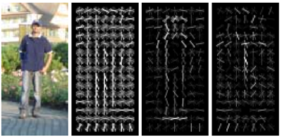Dalal-Triggs focuses on representation more than learning and introduces the SIFT-like Histogram of Gradients (HoG) representation (pictured to the right). You will not be asked to implement HoG. You will be responsible for the rest of the detection pipeline -- handling heterogeneous training and testing data, training a linear classifier, and using your classifier to classify millions of sliding windows at multiple scales. Fortunately, linear classifiers are compact, fast to train, and fast to execute. A linear SVM can also be trained on large amounts of data, including mined hard negatives.

Details and Starter Code

The following is an outline of the stencil code (see links for provided code and VLFeats library download above):

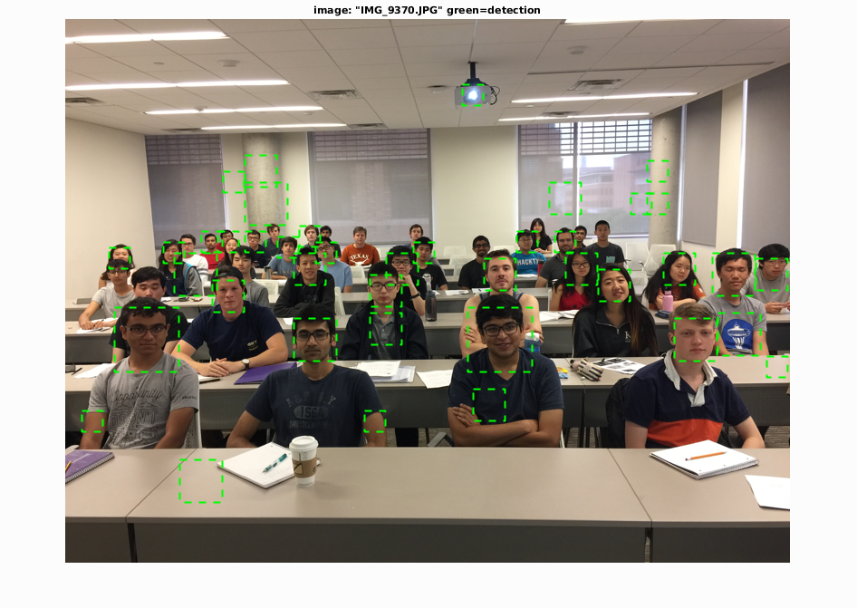
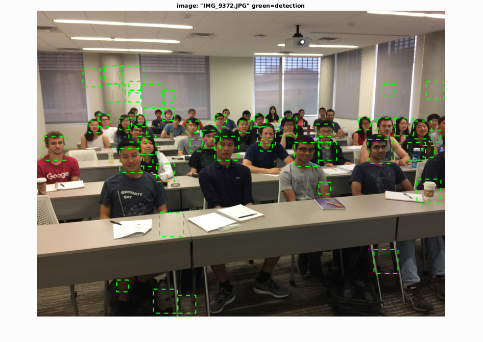
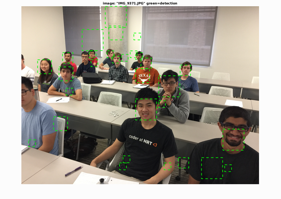
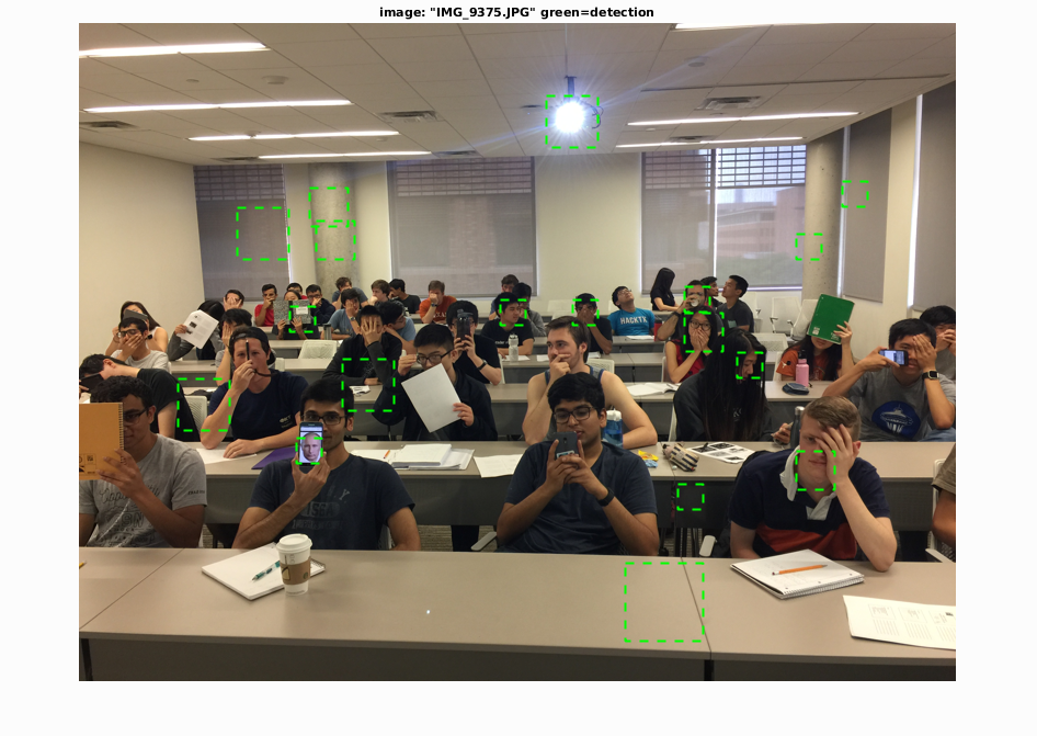
• proj4.m. The top level script for training and testing your object detector. If you run the code unmodified, it will predict random faces in the test images. It calls the following functions, many of which are simply placeholders in the starter code:
• get_positive_features.m (you code this). Load cropped positive trained examples (faces) and convert them to HoG features with a call to vl_hog.
• get_random_negative_features.m (you code this). Sample random negative examples from scenes which contain no faces and convert them to HoG features.
• classifier training (you code this). Train a linear classifier from the positive and negative examples with a call to vl_trainsvm.
• run_detector.m (you code this). Run the classifier on the test set. For each image, run the classifier at multiple scales and then call non_max_supr_bbox to remove duplicate detections.
• evaluate_detections.m. Compute ROC curve, precision-recall curve, and average precision. You're not allowed to change this function.
• visualize_detections_by_image.m. Visualize detections in each image. You can use visualize_detections_by_image_no_gt.m for test cases which have no ground truth annotations (e.g. the class photos).

Creating the sliding window, multiscale detector is the most complex part of this project. It is recommended that you start with a single scale detector which does not detect faces at multiple scales in each test image. Such a detector will not work nearly as well (perhaps 0.3 average precision) compared to the full multi-scale detector. With a well trained multi-scale detector with small step size you can expect to match the papers linked above in performance with average precision above 0.9.

Data

The choice of training data is critical for this task.  Face detection methods have traditionally trained on heterogeneous, even proprietary, datasets. As with most of the literature, we will use three databases: (1) positive training crops, (2) non-face scenes to mine for negative training data, and (3) test scenes with ground truth face locations.

You are provided with a positive training database of 6,713 cropped 36x36 faces from the Caltech Web Faces project. This subset has already filtered away faces which were not high enough resolution, upright, or front facing. There are many additional databases available For example, see Figure 3 in Huang et al. and the LFW database described in the paper. You are free to experiment with additional or alternative training data for extra credit.

Non-face scenes, the second source of your training data, are easy to collect. You are provided with a small database of such scenes from Wu et al. and the SUN scene database. You can add more non-face training scenes, although you are unlikely to need more negative training data unless you are doing hard negative mining for extra credit.

The most common benchmark for face detection is the CMU+MIT test set. This test set contains 130 images with 511 faces. The test set is challenging because the images are highly compressed and quantized. Some of the faces are illustrated faces, not human faces. For this project, we have converted the test set's ground truth landmark points in to bounding boxes. We have inflated these bounding boxes to cover most of the head, as the provided training data does. For this reason, you are arguably training a "head detector" not a "face detector" for this project.

Copies of these data sets are provided with your starter code linked above in Resources.   Please do not include them in your submission on Canvas.

Write up

In the report, please include the following:

• Describe your algorithm and any decisions you made to write your algorithm a particular way.
  
• Show and discuss the results of your algorithm.
  
• Discuss any extra credit you did, and clearly show what contribution it had on the results (e.g. performance with and without each extra credit component).
• Show how your detector performs on additional images in the data/extra_test_scenes directory.
• Include the precision-recall curve and AP of your final classifier and any interesting variants of your algorithm.

Face detection contest

There will be extra credit and recognition for the students who achieve the highest average precision, whether with the baseline classifier or any bells and whistles from the extra credit.   You aren't allowed to modify evaluate_all_detections.m which measures your accuracy.

Extra Credit

For all extra credit, be sure to analyze in your report cases where your extra credit implementation has improved classification accuracy. Each item is "up to" some amount of points because trivial implementations may not be worthy of full extra credit.  A maximum of 20 extra credit points are allowable.

Some ideas:

• up to 5 pts: Implement hard negative mining, as discussed in the Dalal and Triggs paper, and demonstrate the effect on performance.
• up to 10 pts: Implement a cascade architecture as in Viola-Jones. Show the effect that this has on accuracy and run speed. Describe your cascade building process in detail in your handout. Unfortunately, with the current starter code this is unlikely to improve run speed because the run time is dominated by image and feature manipulations, not the already fast linear classifier.
• up to 10 pts: Detect additional object categories. You'll need to get your own training and testing data. One suggestion is to train and run your detector on the Pascal VOC data sets, possibly with the help of their support code. The bounding boxes returned by the stencil code are already in VOC format.
• up to 5 pts: Find and utilize alternative positive training data to improve results. You can either augment or replace the provided training data.
• up to 10 pts: Add contextual reasoning to your classifier. For example, one might learn likely locations of faces given scene statistics, in the spirit of Contextual priming for object detection, Torralba. You could try and use typical arrangements of groups of faces as in Understanding Images of Groups of People and Finding Rows of People in Group Images by Gallagher and Chen.
• up to 5 pts: Experiment with alternative features or additional features to improve accuracy.
  

For any of the above, be sure to explain clearly in your report --- with quantitative results wherever relevant --- the outcomes via experiments.

Handing in

Creating a single zip file to submit on Canvas.  It should contain the following:

• README - text file containing anything about the project that you want to tell the TA
• code/ - directory containing all your code for this assignment
• report.pdf - writeup as described above. 
  
• Be sure to prominently show your average precision results from evaluate_all_detections.m
  on the test set for the sake of the contest.
  

Do NOT submit the provided data within your zip file.  The TA will have a local copy.

How grades will be calculated

• +20 pts: Use the training images to create positive and and negative training HoG features.
• +15 pts: Train linear classifier.
• +45 pts: Create a multi-scale, sliding window object detector.
• +20 pts: Writeup with design decisions and evaluation.
• +20 pts: Extra credit (up to 20 points)

Advice, Tips

• Read the comments in the provided code.
• The starter code has more specific advice about the necessary structure of variables through the code. However, the design of the functions is left up to you. You may want to create some additional functions to help abstract away the complexity of sampling training data and running the detector.
• You are free to play with any parameters.  To give a starting point, HoG cell sizes of 6 are reasonable.  Positive patch sizes of 36 x 36 pixels (as given in the code) are reasonable.  Negative patch sizes of 36 x 36, 48 x 48, 72 x 72, sampled with step sizes of 48 are reasonable as a starting point.
  
• You probably don't want to run non-max suppression while mining hard-negatives (extra credit).
• While the idea of mining for hard negatives is ubiquitous in the object detection literature, on this testbed it may only modestly increase your performance when compared to a similar number of random negatives.
• The parameters of the learning algorithms are important. The regularization parameter lambda is important for training your linear SVM. It controls the amount of bias in the model, and thus the degree of underfitting or overfitting to the training data. Experiment to find its best value.
• Your classifiers, especially if they are trained with large amounts of negative data, may "underdetect" because of an overly conservative threshold. You can lower the thresholds on your classifiers to improve your average precision. The precision-recall metric does not penalize a detector for producing false positives, as long as those false positives have lower confidence than true positives. For example, an otherwise accurate detector might only achieve 50% recall on the test set with 1000 detections. If you lower the threshold for a positive detection to achieve 70% recall with 5000 detections your average precision will increase, even though you are returning mostly false positives.
• When coding run_detector.m, you will need to decide on some important parameters. (1) The step size. By default, this should simply be the pixel width of your HoG cells. That is, you should step one HoG cell at a time while running your detector over a HoG image. However, you will get better performance if you use a fine step size. You can do this by computing HoG features on shifted versions of your image. This is not required, though -- you can get very good performance with sampling steps of 4 or 6 pixels. (2) The step size across scales, e.g. how much you downsample the image. A value of 0.7 (the image is downsampled to 70% of it's previous size recursively) works well enough for debugging, but finer search with a value such as 0.9 will improve performance. However, making the search finer scale will slow down your detector considerably.
• Likewise your accuracy is likely to increase as you use more of the training data, but this will slow down your training. You can debug your system with smaller amounts of training data (e.g. all positive examples and 10000 negative examples).
• You can train and test a classifier with average precision of 0.85 in about 60 seconds. It is alright if your training and testing is slower, though.  5-10 minutes is not unreasonable.
  
• The Viola-Jones algorithm achieves an average precision of 0.895* on the CMU+MIT test set based on the numbers in Table 3 of the paper (This number may be slightly off because Table 3 doesn't fully specify the precision-recall curve, because the overlap criteria for VJ might not match our overlap criteria, and because the test sets might be slightly different -- VJ says the test set contains 507 faces, whereas we count 511 faces). You can beat this number, although you may need to run the detector at very small step sizes and scales. We have achieved Average Precisions around 0.93.

Credits

This project is based on the one originally created by Prof. James Hays of Georgia Tech, who kindly gave us permission to use his project description and code.   Figures in this handout are from Dalal and Triggs.  Thanks also to Chao-Yeh Chen for performing a trial run of the assignment.

We tried to make especially easy test cases with neutral, frontal faces.

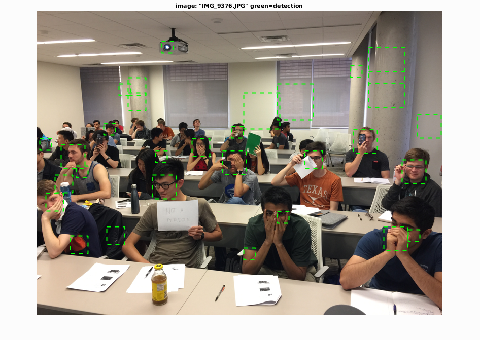The CS 378H class demonstrates how not to be seen by a robot.