Learning a Hierarchy of Discriminative Space-Time Neighborhood Features for Human Action Recognition
Adriana Kovashka and Kristen Grauman
University of Texas at Austin
Summary
Recent work shows how to use local spatio-temporal features to learn models of realistic human actions from video. However, existing methods typically rely on a predefined spatial binning of the local descriptors to impose spatial information beyond a pure "bag-of-words" model, and thus may fail to capture the most informative space-time relationships. We propose to learn the shapes of space-time feature neighborhoods that are most discriminative for a given action category. Given a set of training videos, our method first extracts local motion and appearance features, quantizes them to a visual vocabulary, and then forms candidate neighborhoods consisting of the words associated with nearby points and their orientation with respect to the central interest point. Rather than dictate a particular scaling of the spatial and temporal dimensions to determine which points are near, we show how to learn the class-specific distance functions that form the most informative configurations. Descriptors for these variable-sized neighborhoods are then recursively mapped to higher-level vocabularies, producing a hierarchy of space-time configurations at successively broader scales. Our approach yields state-of-the-art performance on the UCF Sports and KTH datasets.
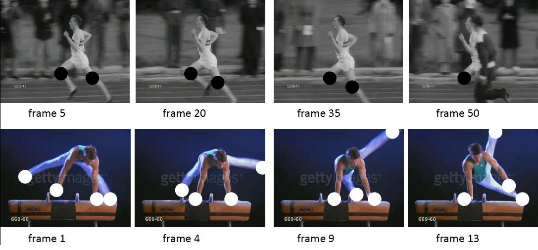
Figure 1: The most discriminative space-time neighborhoods of local descriptors (denoted by circles) may depend on the activity category. For example, for running (first row) a larger temporal extent and smaller spatial extent is most useful, whereas for swinging (second row), the reverse is true. The main idea of the proposed method is to learn class-specific vocabularies of variable-shaped space-time neighborhoods.
Approach
Outline:
Extract raw features (level-0 features) and form level-0 vocabulary.
Form space-time neighborhoods (level-1 features), reduce dimensionality with PCA, and form level-1 vocabulary.
Form a hierarchy of neighborhoods.
Repeat for different distance scalings and pick the discriminative scalings for each class with MKL.
Compute chi-squared kernels for training and apply SVM for recognition.
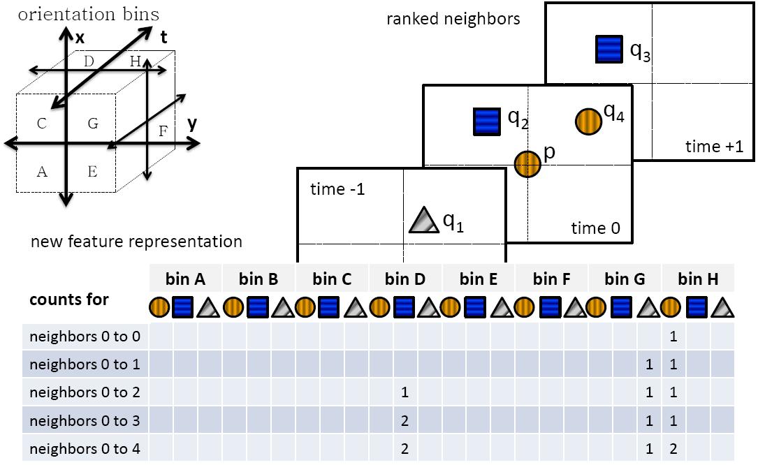
We use the HoG/HoF features described by Laptev et al. for our sparse features, extracted using the method by Laptev, and HoG3D for our densely sampled features (Kläser et al.). Then we form neighborhoods of these points, using each point as a center of a neighborhood. For each of the N nearest neighbors, we record its orientation with respect to the central point, as well as its correspondence to a "level-0" visual word (which was computed on the basic raw interest point level).
Figure 2: Neighborhood formation overview. The 3d axes in the upper-left depict the 8 orientations relative to the central point. Each letter denotes a space-time orientation. In the center, we depict three frames with their features and corresponding visual words (shapes represent word identity). The histogram at the bottom is our neighborhood representation. For example, neighbor 1 (q_1) is (G=above, right, and before) the central feature p, and its word is of type "triangle", so we increment the bin for word "triangle" and orientation G in the first row. We also increment the count in the cells directly below, recording the neighbors cumulatively.
Now the histogram depicted in Figure 2 is reshaped to a vector and becomes the new representation of the central feature. We can now form a "level-1" vocabulary using these new features.
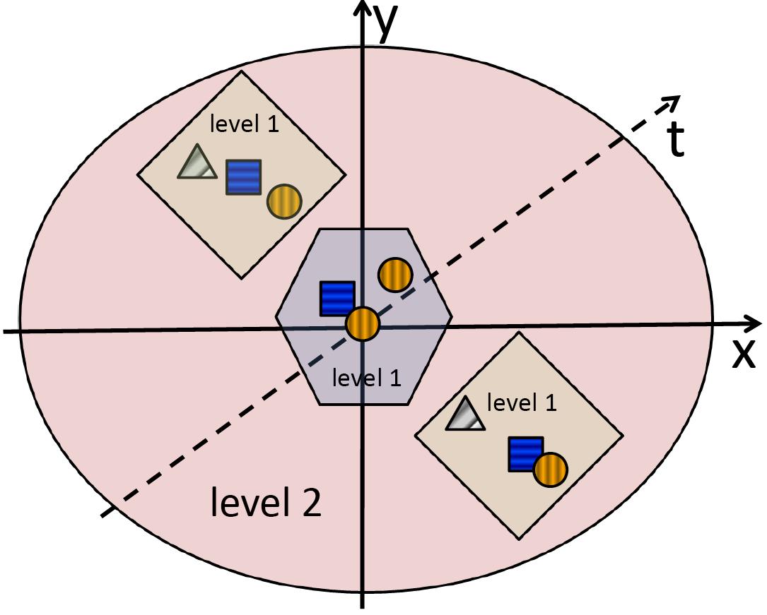
We can repeat this neighborhood formation to form higher-level vocabularies, as shown in Figure 3. In our experiments, we stopped at "level-2" (for 3 levels total, including the base level).
Figure 3: Illustration of the feature / vocabulary hierarchy. The hexagon and diamonds are level-1 visual words composed of level-0 words. The red ellipse is a level-2 word composed of level-1 words (here N=3).
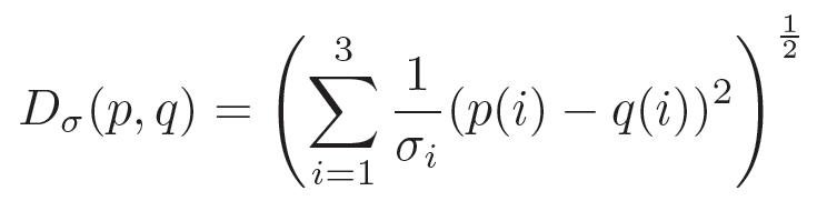
In the realm of space-time neighborhoods, we need to resolve the problem of scaling the space and time dimensions because a unit of one pixel is not necessarily equivalent of a unit of one frame. Therefore, we learn a Mahalanobis distance in the form of a diagonal covariance matrix, as defined in Equation 1. We compute different values for σ and use Multiple Kernel Learning (MKL) to learn the useful x, y, t combinations. We use the code by Obozinski for MKL.
Equation 1
Figure 4: Examples of level-1 words. The most relevant word for the hand-clapping (top) and horse-riding (bottom) actions, as determined by mutual information. (To save space, we omit some intermediate frames).
To train an SVM, we use the chi-squared distance. We compute one kernel for each of our F(ML+1) channels, where F is the number of feature types, M is the number of x, y, t combinations, and L is the number of non-base vocabulary levels.
Results
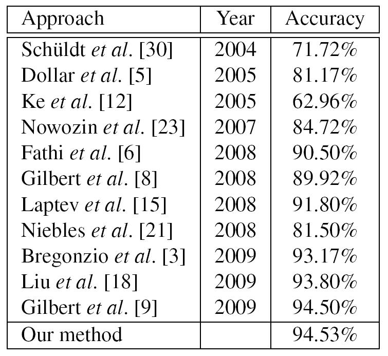
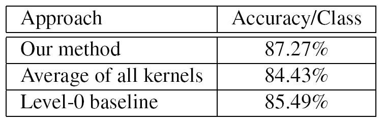
We obtain state-of-the-art results on two benchmark datasets, KTH and UCF Sports.
Figure 5: Comparison of recogniton accuracy on the KTH dataset.
Figure 6: Results on the UCF Sports dataset.
Finally, we present some visualization of the recognition performance, as well as the features at different vocabulary levels.
Figure 7: Probabilities for the different classes on the UCF Sports datasest. Training was done in one-vs-all fashion, and the maximum probability from the 10 one-vs-all runs, each corresponding to one of the 10 classes, was taken to label a given video.
level 0
level 1
level 2
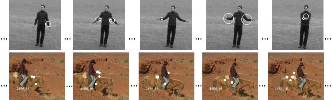
Figure 8: Some level-0, level-1, and level-2 features (formed from the same central points) in one UCF video. Different colors denote different features / neighborhoods. Also note that the ellipses have been scaled up by a factor of 5 in order to be more clearly visible. Each video loops 10 times.
Implementation note: Please note that in Equation 1 in our paper, the term 1/σ_i should have been squared to match our actual implementation. The correct values for 1/σ_i that correspond to Equation 1 as presented in the paper are: 1/σ_i = {1, 25, 100, 2500} for KTH and 1/σ_1 = 1, 1/σ_2 = 1/σ_3 = {1, 100} for UCF.
Publication
Learning a Hierarchy of Discriminative Space-Time Neighborhood Features for Human Action Recognition. Adriana Kovashka and Kristen Grauman. To appear, Proceedings of the IEEE Conference on Computer Vision and Pattern Recognition (CVPR), San Francisco, CA, June 2010. [pdf][poster]