Boundary Preserving Dense Local
Regions
Jaechul Kim and Kristen Grauman
Motivation
Good features to match images: Repeatable
across the images and distinctive
among the features.
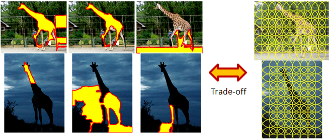
Distinctive but not repeatable (Segmented
regions)
Repeatable
but
not distinctive (Dense patch sampling)
Figure
1. Trade-off of distinctiveness and repeatability of existing features.
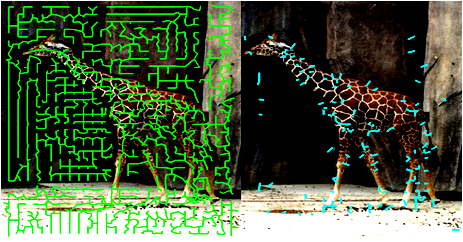
Boundary Preserving Local Regions (BPLRs)
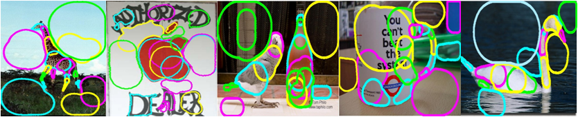
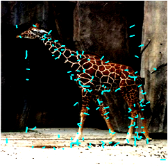
Figure
2. Example detections of BPLRs.
- BPLRs respect object boundaries, capturing object's local shape.
- BPLRs are densely extracted in a regular grid across the image,
although Figure 2 shows only a fraction of extracted regions for
display.
- Dense and shapre-preserving properties make BPLRs both repeatble and distinctive.
- To obtain BPLRs, we propose a novel feature sampling and linking
strategy driven by multiple segmentation.
BPLR's Key Contrast
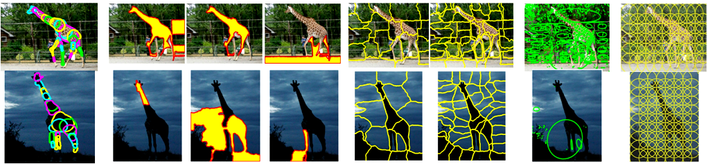
(a)
BPLR
(b)
Segmented
regions
(c)
Superpixels
(d)
MSER
(e)
Dense sampling
Figure 3. Illustration of BPLR's key constrasts with representative
existing detectors. Existing detectors lack either repeatability or
distinctiveness, or even both. On the other hand,
the proposed BPLRs captures object’s local shape in a repeatable
manner under image variation like appearance and background
clutter. (Note, for BPLRs we display only a sample
for different foreground object parts; our complete extraction is
dense and covers entire image.)
Approach
- Overview
Our method consists of three major components: 1) sampling base
features, which we call "elements",
from
each
segment of a pool of multiple segmentations,
2) linking the sampled elements into a single graph across the
image, and 3) grouping neighbor elements in the graph to form BPLRs.
Initial elements for one
segment
Minimum spanning tree
Edge
removed
Grouped
elements
--> One BPLR -->
Descriptor
(a)
Sampling elements
(b) Linking elements across the image
(c) Grouping neighbor elements
into BPLRs
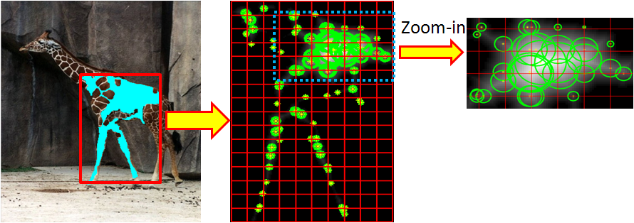
Figure 4. Main components of the approach. (a) For each initial
segment from a pool of multiple segmentations, we sample local
elements densely in a grid according to its distance transform
(left: segment; lower right: grid; upper right: zoom-in to show
sampled elements and their scales). (b) Elements are linked across
the image, using the overlapping multiple segmentations to create
a single structure that reflects the main shapes and segment layout.
(c) Using that structure, we extract one BPLR per element. Each BPLR
is a group of neighboring elements. Finally, the BPLR
is mapped to some descriptor (we use PHOG+gPb).
- Sampling
The first step of our method is to sample elements from each segment
of the input segmentations.
Given a segment, we compute distance transform from the boundary of
the segment and divide the segment into regular grid cells.
At each grid cell, we sample an element at the location with the
maximal distance transform value within the cell (Figure 5 (b)).
The sampled element is represented by a circle; its center is the
sampled location and its radius, the element's scale, is given by
that maximal distance transform value at the sample position (Figure
5(c)).
Our distance transform (DT)-based sampling has two geometric
properties:
- First, elements' scales by DT values prevents elements from
overlapping segment's boundary (boundary preserving).
- Second, refining the dense sampling positions by the maximal
DT values pushes sampled locations to the inner part of each
segment (concentrating effect).
- This concentrating effect keeps elements originating from
the same segment closer to one another than those from
different segments, giving a soft preference to join elements
originating from the same segment in the linking stage next.
(a)
One
segment
(b)
Sampling at dense
grids
(c)
Zoom-in view of sampled elements
Figure
5. Sampling elements in a segment.
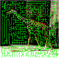
- Linking
Given sampled elements from all
segments, we link them into a single graph structure. We
compute a global linkage graph connecting all element locations via
a minimum spanning tree,
where each edge weight is given by the Euclidean distance between
the two points it connects. By minimizing the sum of total edge
weights, the resulting spanning tree removes
the longer edges from the graph—most of which cross object
boundaries due to the "concentrating effect" of the DT-based
sampling (Figure 6(a)).
Note, although our linking method favors linkages among same-segment
elements, linkages are not restricted to each single segment by
overlapping multiple segments.
Whereas the minimum spanning tree reduces connectivity for more
distant elements, we also want to reduce connectivity for elements
divided by any apparent object contours.
Thus, in the second linkage step, we compute a simple
post-processing of the spanning tree that removes noisy tree edges
that cross strong intervening contours (we use gPb for contour
detection).
Figure 6(b) shows the types of links removed by this
post-processsing; we see that most do indeed cross object
boundaries.
(a) Minimum spanning
tree
(b)
Spurious
tree edges removed by post-processing
Figure
6. Linking elements across the image
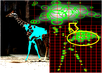
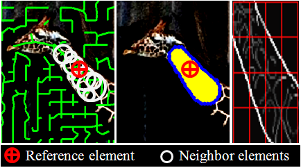
- Grouping
Finally, we group neighbor elements for
each element in the graph, which forms BPLR
of the element.Given an element, we define its
topological neighbors within N
hops from the element.
And, we also
define its Euclidean neighbors within F times the scale of the element. Intersection
of topological and Euclidean neighbors forms a BPLR of the
element, and we represent a BPLR with a descriptor.
Any existing
descriptors can be used; in our experiment we used PHOG with gPb
edge for descriptor.We repeat the same procedure for all
elements in the graph, obtaining dense extraction of BPLRs.
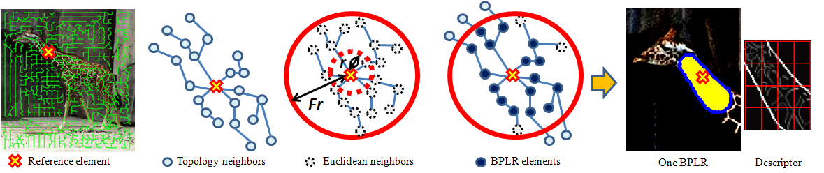
Figure 7. Grouping neighbor elements into a BPLR for a reference
element. Topology neighbors: up to
N(= 3) hops for the reference; Euclidean neighbors: within
F times the scale of the
reference;
BPLR elements: intersection of topology and Euclidean neighbors.
Every extracted BPLR is represented by a descriptor, for which we
use PHOG + gPb in the experiment.
Results
We made experiments to evaluate raw feature quality of BPLR compared
to existing feature detectors.
Then we apply it to foreground discovery and object classification
to show its effectiveness when used for tasks that require reliable
feature matching.
- Repeatability
First, we test repeatability of
feature for
object category matching. To measure repeatability, we use Bounding Box Hit Rate - False
Positive Rate (BBHR-FPR) metric introduced by Quack
et.al.
It
evaluates how well foreground
features on an object match other foreground features in the same class.
We compare BPLR to existing region detectors, including dense
sampling, local interest operator (MSER), and segmented regions.
In
addition, we compare BPLR to semi-local features which use
class-specific supervision to find geometric configurations of
local features common to the class.
Figure 8 and 9 show BPLR outperforms all the baselines.
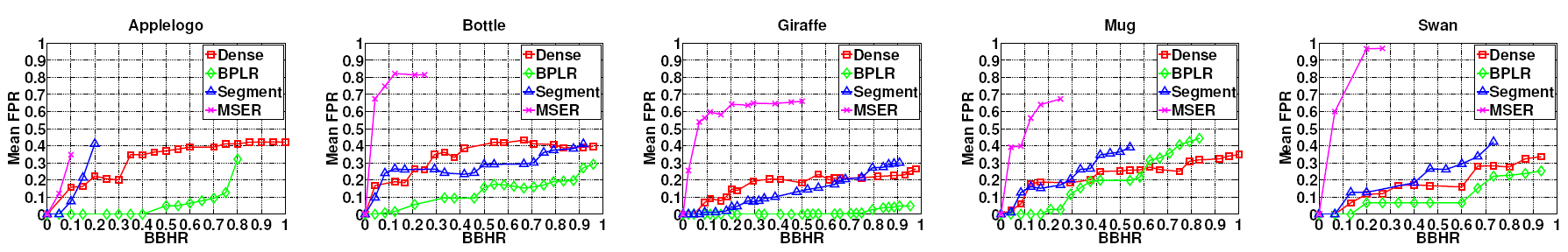
Figure 8. Repeatability on ETHZ shape objects. Plots compare BPLR to
three alternative region detectors: MSER, dense sampling, and
segments. Quality is measured by the bounding box hit rate-false
positive rate (BBHR-FPR).
Curves that are lower on the y-axis (fewer false positives) and
longer along the x-axis (higher hit rate) are better.
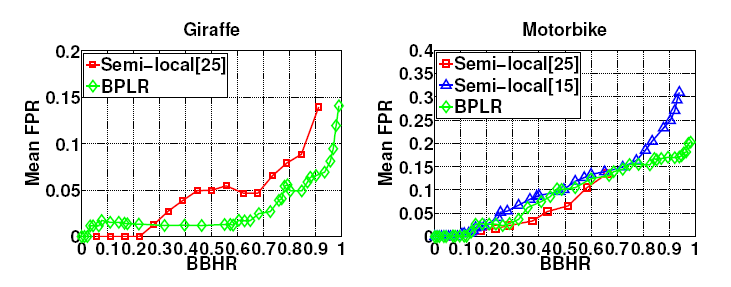
Figure 9. Repeatability on ETH+TUD objects. Plots compare BPLR to
two state-of-the-art semi-local feature methods [25, 15].
([15] does not report results on the Giraffe class.)
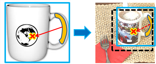
- Localization Accuracy
Second, we evaluate
localization accuracy of feature matching. To measure
localization accuracy, we introduce Bounding Box Overlap Score - Recall
(BBOS-Recall) metric.
It evaluates how
accurately
feature
matches can predict objects’ positions and scale as shown in
Figure 10.
Training
image
Test image
Figure 10. Given two matched regions and their relative scales, we
project the training exemplar’s bounding box into the test image
(dotted rectangle).
That match’s BBOS is the overlap ratio between the projected box and
the object’s true bounding box.
In Figure 11, we see BPLR provides better localization
accuracy, verifying the distinctiveness of BPLR by capturing
object’s local shape.
In addition, Figure 12 shows example matches of BPLR, illustrating
BPLR's localization power. In this example, we automatically select the top
five non-overlapping regions based on the nearest-neigbor matching
distance.
Leftmost image at each row is the test image and
remaining images are training images which have the best matches
for the test BPLRs. Same colors indicate matched
regions.
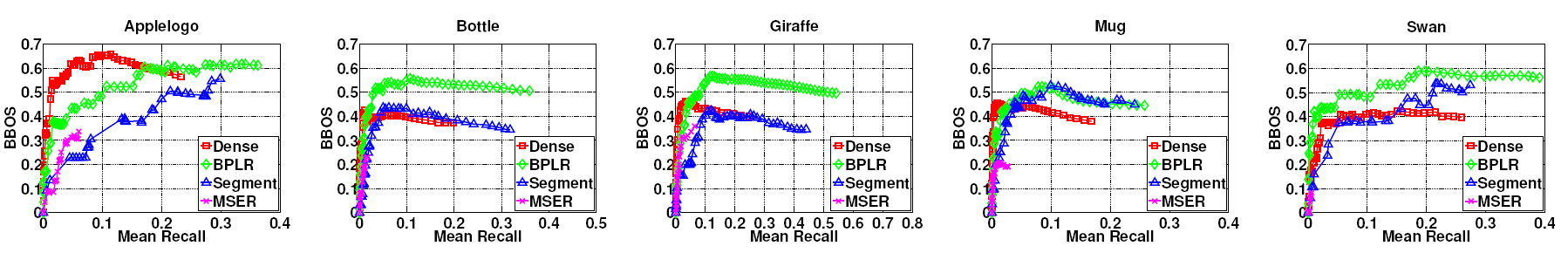
Figure 11. Localization accuracy on ETHZ shape objects. Plots
compare our approach (BPLR) to three alternative region detectors:
MSER, dense sampling, and segments. Quality is measured by the
bounding box overlap score - recall (BBOS-Recall),
which captures the layout of the feature matches. Curves that are
higher in the y-axis (better object overlap) and longer along the
x-axis (higher recall) are better.
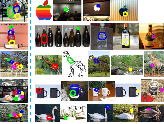
Figure 12. Example matches showing BPLR’s localization accuracy.
Colors in the same row indicate matched regions.
- Foreground Discovery
We apply BPLR to weakly-supervised
foreground discovery, in which the system is given a set of
cluttered images that all contain the same object class,
and must estimate which pixels are foreground.
In
this experiment, we aim to show that BPLR is effective for
segmentation in place of superpixels, which is widely used for
segmentation.
For
foreground discovery, we implement GrabCut where we replace
superpixels by BPLRs and use BPLR matching scores to estimate the
foreground.
Our
BPLR-based GrabCut implementation achieves the state-of-the-art
performance.
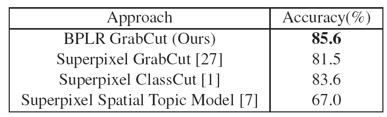
Table 1. Foreground discovery results, compared to several
state-of-the-art methods. Using BPLR regions with a GrabCut-based
solution, we obtain
the best accuracy to date on the Caltech-28 dataset.
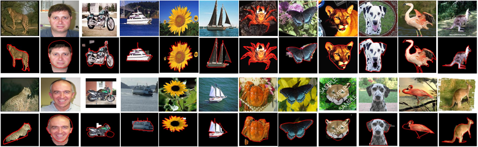
Figure
13. Example foreground discovery results using BPLRs. Two examples per
class. Ground truth is marked in red.
- Object Classification
Lastly, we apply our features to
object recognition on the Caltech-101. We employ a relatively
simple classification model on top of the BPLRs, to help isolate
their
impact. Specifically, we use the Naive Bayes Nearest-neighbor
(NBNN) classifier by Boiman et.al.
Table 2 compares BPLR to alternative feature extractors using NBNN
with identical parameter settings. BPLRs outperforms the baselines.
Table 3 compares to existing nearest neighbor-based results: we
are among the leading accuracy. BPLRs outperforms the baselines.BPLRs outperforms the
baselines.
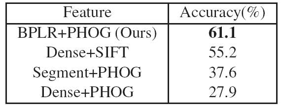
Table 2.
Direct comparison of BPLR to other feature detectors on the
Caltech-101 (15-15 training/test images).
The only thing varying per method is the feature extractor,
and our method provides the most accurate results.
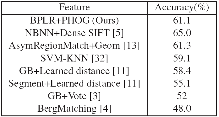
Table 3. Comparison to existing results on the Caltech-101 that
use nearest neighbor-based classifiers.
Conclusions
We
proposed a novel segmentation-driven feature sampling and
linking strategy to produce repeatable shape-preserving local
regions. As shown through extensive experiments, the key
characteristics that distinguish BPLR from existing detectors
are:
- it can improve the ultimate descriptors’
distinctiveness, while still retaining thorough coverage
of the image,
- it exploits segments’ shape cues without relying on them
directly to generate regions, thereby retaining robustness
to segmentation variability, and
- its generic bottom-up extraction makes it applicable
whether or not prior class knowledge is available.
Publication
Jaechul
Kim and Kristen Grauman, Boundary Preserving Dense Local
Regions, In Proc. International Conference on
Computer Vision and Pattern Recognition (CVPR), Jun.
2011. [pdf] [slides]
Code
To download the code, you can check out this page: [code download]